3D Deconvolution for Low Photon Count Fluorescence Imaging | Scientific Reports 2018

Hayato Ikoma, Michael Broxton, Takamasa Kudo, Gordon Wetzstein

A convex algorithm 3D deconvolution of low photon count fluorescence imaging.

ABSTRACT

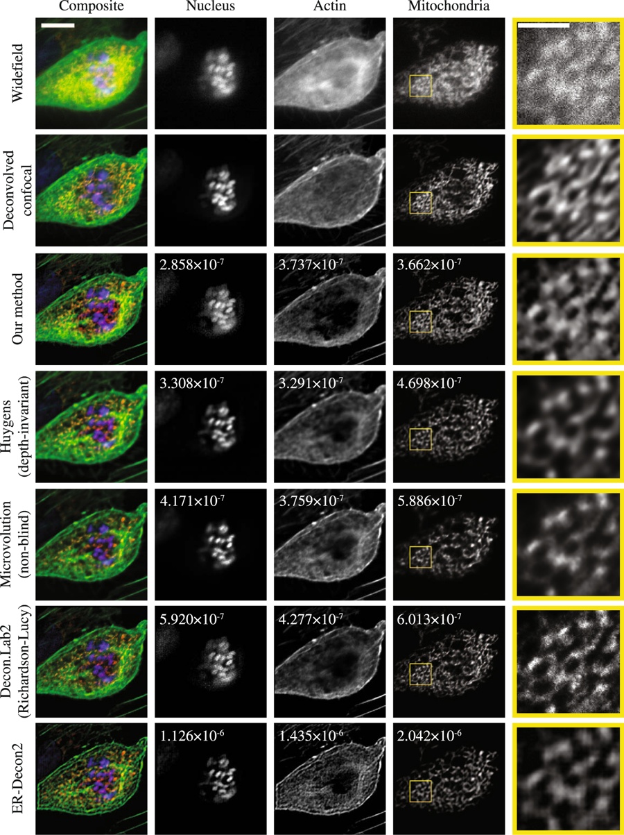
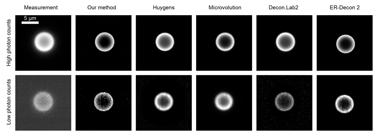
Deconvolution is widely used to improve the contrast and clarity of a 3D focal stack collected using a fluorescence microscope. But despite being extensively studied, deconvolution algorithms can introduce reconstruction artifacts when their underlying noise models or priors are violated, such as when imaging biological specimens at extremely low light levels. In this paper we propose a deconvolution method specifically designed for 3D fluorescence imaging of biological samples in the low-light regime. Our method utilizes a mixed Poisson-Gaussian model of photon shot noise and camera read noise, which are both present in low light imaging. We formulate a convex loss function and solve the resulting optimization problem using the alternating direction method of multipliers algorithm. Among several possible regularization strategies, we show that a Hessian-based regularizer is most effective for describing locally smooth features present in biological specimens. Our algorithm also estimates noise parameters on-the-fly, thereby eliminating a manual calibration step required by most deconvolution software. We demonstrate our algorithm on simulated images and experimentally-captured images with peak intensities of tens of photoelectrons per voxel. We also demonstrate its performance for live cell imaging, showing its applicability as a tool for biological research.

CITATION

H. Ikoma, M. Broxton, T. Kudo, G. Wetzstein. “A convex 3D deconvolution algorithm for low photon count fluorescence imaging”, Scientific Reports, 2018.

BibTeX

@article{Ikoma:2018:3Ddeconvolution,
author = {Hayato Ikoma and Michael Broxton and Takamasa Kudo and Gordon Wetzstein},
title = {A convex 3D deconvolution algorithm for low photon count fluorescence imaging},
journal = {Scientific Reports},
year = {2018},
}


Acknowledgements

We thank Dr. Jon Mulholland and Dr. Cedric Espanel at the Cell Sciences Imaging Facility at Stanford University for their help on capturing datasets. We also thank Dr. Aurélien Bourquard for his advice about the use of the Hessian-based regularizer. This project was generously supported by Olympus, a Sloan Research Fellowship, an NSF CAREER award (IIS 1553333), and by the NSF/Intel Partnership on Visual and Experiential Computing (Intel #1539120, NSF #IIS1539120).

ADDITIONAL MATERIAL

Composite image showing raw measurements (lower left) and processed data (upper right) for a live cell experiment.


Varying perspectives of deconvolution results for imaging of live cells expressing histone H2B fused to mClover to visualize chromosome conformation.

Time sequence of deconvolution results for imaging of live cells expressing histone H2B fused to mClover to visualize chromosome conformation.


Deconvolution results for imaging of live cells expressing histone H2B fused to mClover to visualize chromosome conformation. (a) A focal stack (512 × 512 × 128 voxels) of the cell was captured over a span of one and a half hours with a time interval between focal stacks of three minutes. The 49-th z slice of the measurement, the deconvolved volume using our method, and the deconvolved volume using the Richardson-Lucy algorithm (100 iterations) is shown, with the time interval of fifteen minutes between frames along each row. (b) A second focal stack (512 × 512 × 100 voxels) shows a cell recorded for one hour with a time interval of three minutes. The 37-th z slice is shown, and the time interval between frames in each row is fifteen minutes. The corresponding deconvolved images are visualized in the second and third rows, respectively. The scale bar has the length of 10 μm. 3D volume renderings of these cells are provided as Supplementary Videos 3 and 4.


A comparison of 3D deconvolution software used to process a low SNR, 512 × 512 × 22 voxel widefield fluorescence focal stack. The focal stack was captured with three color channels (the first row) and then deconvolved with six deconvolution software methods (rows three through eight). The second row shows a confocal microscope image deconvolved with the Huygens software as a baseline for comparison. The fifth column shows the magnified image of the yellow rectangle in the corresponding mitochondria image. The composite images (the first column) show the sixth z slice of a pseudo-colored 3D image combining the three color channels. The nucleus, actin and mitochondria images (the second, third and fourth columns) show the eleventh, fourth and sixth z slice of the deconvolved 3D images. The scale bar in the composite image is 10 μm, and the scale bar in the magnified image is 3 μm. The number written in the figures are the minimum NMSE measured when comparing these data to deconvolved confocal images. All XY slices of the focal stacks are shown in a sequence in Supplementary Video 2.


Deconvolution results for experimentally captured focal stacks containing a 6 μm hollow microsphere