Overview
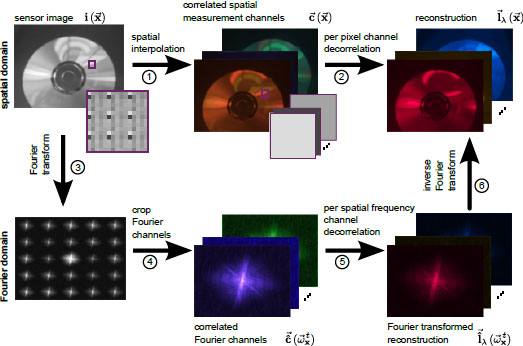
Overview of multiplexed image reconstruction. The plenoptic function can be reconstructed by interpolating all measurement channels and performing a local decorrelation in the spatial domain (upper row). Alternatively, it can be reconstructed in the Fourier domain by cropping and locally decorrelating the Fourier channels created by the plenoptic modulator (lower row). This schematic illustrates our mathematical framework that unifies many previously proposed multiplexing and corresponding reconstruction approaches.
Case Studies

Multiplexing Color Information. Raw sensor image with magnified part and corresponding CFA (upper left). Fourier transform with channel correlations illustrated for the entire image and the magnified CFA (upper right). Reconstruction of the non-perfectly bandlimited signal in the spatial (lower left) and Fourier (lower right) domain reveal different aliasing artifacts.
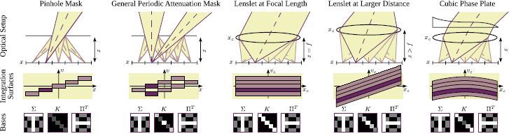
Our theory applied to light field imaging. Columns 1 to 5 illustrate different light field camera configurations (upper row), corresponding integration surfaces in light field space for the individual sensor pixels (center row), and the spatial and plenoptic basis functions (lower row). The convolution of a periodic attenuation mask can be separated into a spatial and plenoptic part using the Fourier basis (column 2). Integration surfaces for refractive optical elements already include the mapping g^-1 from sensor space to camera or world space on the microlens plane.
![Comparison of reconstruction quality for Cones data set (Veeraraghavan et al. [2007]). All results are three-times upsampled during reconstruction. Left: upsampling by zero-padding the 4D inverse FFT. Center: low resolution 4D inverse FFT followed by bicubic upsampling. Right: bicubic up-sampling of correlated measurement channels followed by local decorrelation.](http://www.computationalimaging.org/wp-content/uploads/2017/06/casestudies3.jpg)
Comparison of reconstruction quality for Cones data set (Veeraraghavan et al. [2007]). All results are three-times upsampled during reconstruction. Left: upsampling by zero-padding the 4D inverse FFT. Center: low resolution 4D inverse FFT followed by bicubic upsampling. Right: bicubic up-sampling of correlated measurement channels followed by local decorrelation.
![Comparison of reconstruction quality for Mannequin data set (Lanman et al. [2008]). The results are three-times upsampled and show two different views of the reconstruction, one in each row. First column: upsampling by zero-padding the 4D inverse FFT. Second column: low resolution 4D inverse FFT followed by bicubic upsampling. Third column: bicubic up-sampling of correlated measurement channels followed by local decorrelation. The right-most column shows an example that was computed with a non-linear spatial filter - the joint bilateral filter.](http://www.computationalimaging.org/wp-content/uploads/2017/06/casestudies4.jpg)
Comparison of reconstruction quality for Mannequin data set (Lanman et al. [2008]). The results are three-times upsampled and show two different views of the reconstruction, one in each row. First column: upsampling by zero-padding the 4D inverse FFT. Second column: low resolution 4D inverse FFT followed by bicubic upsampling. Third column: bicubic up-sampling of correlated measurement channels followed by local decorrelation. The right-most column shows an example that was computed with a non-linear spatial filter – the joint bilateral filter.
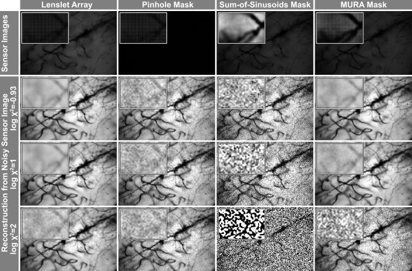
Comparison of noise amplification for different light field acquisition schemes on the golgi stained neuron dataset (lightfield. stanford.edu). The upper row shows simulated sensor images with contrast enhanced close-ups. The other rows show a single view of the reconstructed light field from a noisy sensor image. The ratio chi^2 of signal-dependent photon noise and signal independent dark current noise varies for the different reconstructions. Row 2 simulates a reconstruction with a dominating additive noise term, while rows 3 and 4 show the effect of an increasingly dominating photon noise term in the sensor images.