Learning to Solve PDE-constrained Inverse Problems with Graph Networks | ICML 2022

Qingqing Zhao, David B. Lindell, Gordon Wetzstein

Solving difficult inverse problems in physics using fast GNNs and generative priors.

5 Min Tech Talk

ABSTRACT

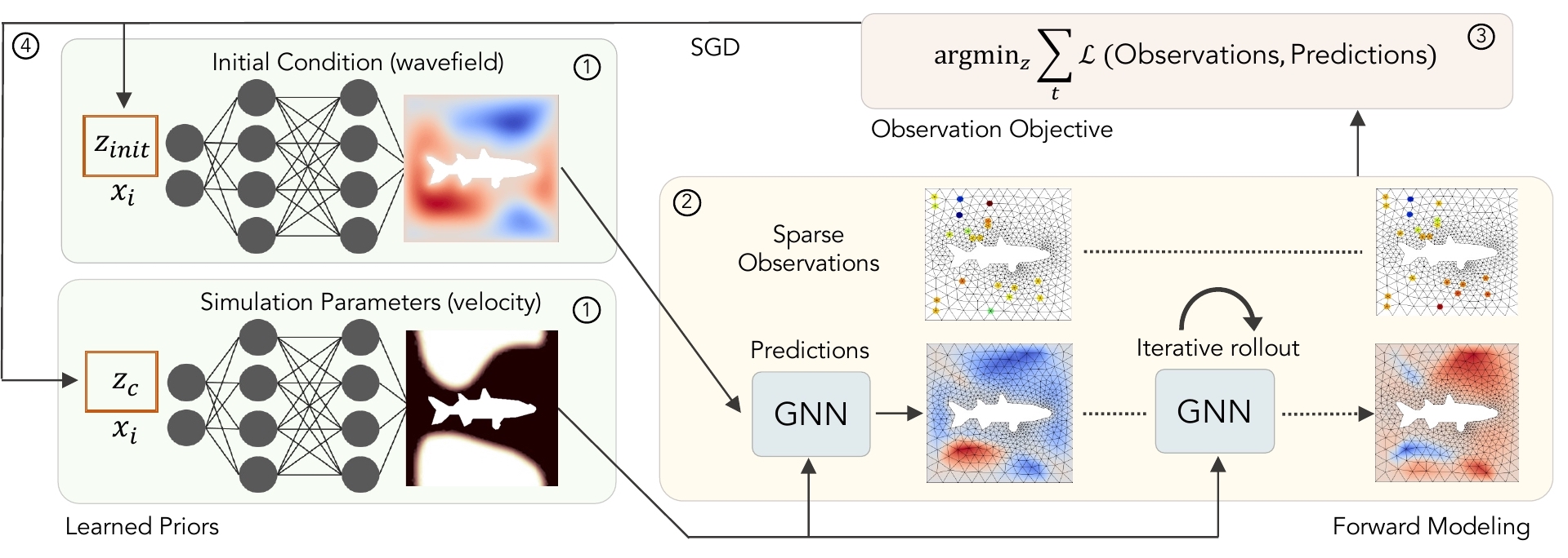
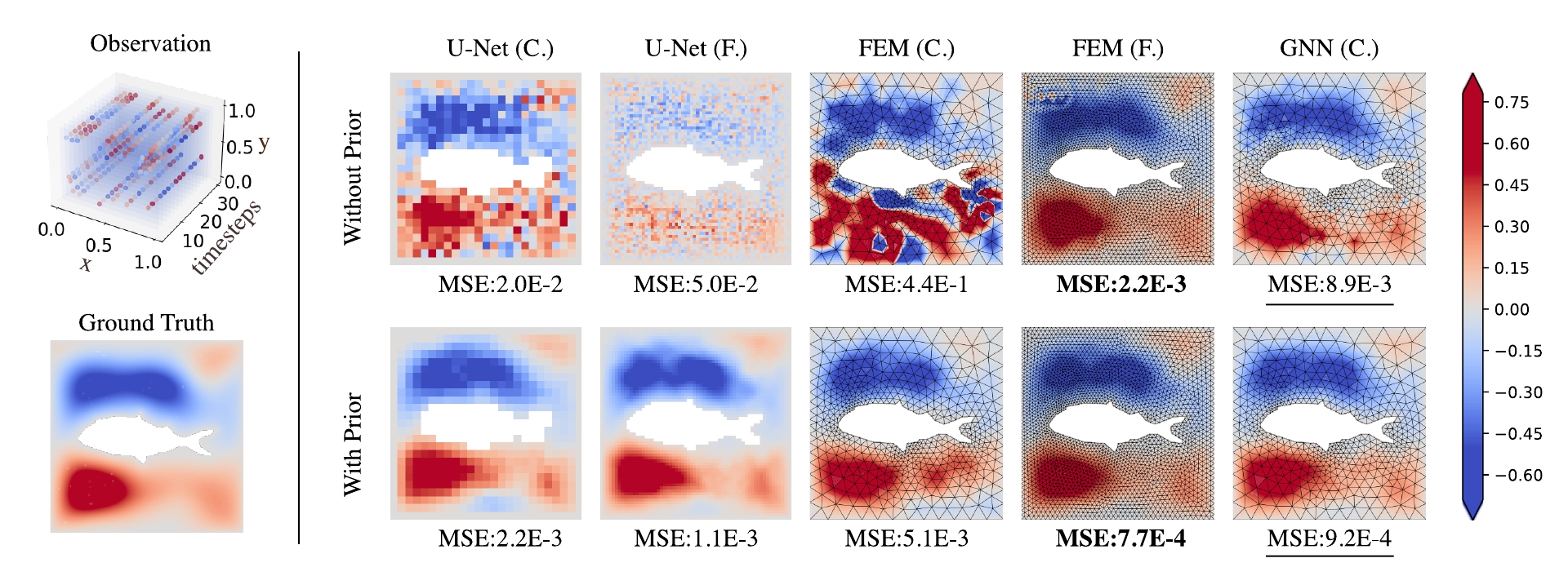
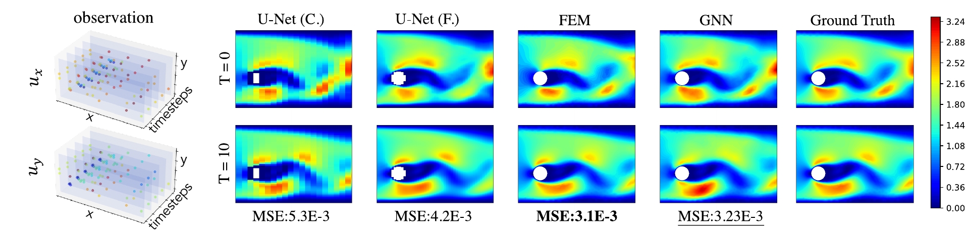
Learned graph neural networks (GNNs) have recently been established as fast and accurate alternatives for principled solvers in simulating the dynamics of physical systems. In many application domains across science and engineering, however, we are not only interested in a forward simulation but also in solving inverse problems with constraints defined by a partial differential equation (PDE). Here we explore GNNs to solve such PDE-constrained inverse problems. Given a sparse set of measurements, we are interested in recovering the initial condition or parameters of the PDE. We demonstrate that GNNs combined with autodecoder-style priors are well-suited for these tasks, achieving more accurate estimates of initial conditions or physical parameters than other learned approaches when applied to the wave equation or Navier-Stokes equations. We also demonstrate computational speedups of up to 90x using GNNs compared to principled solvers.

FILES


CITATION

Q. Zhao, D. B. Lindell, G. Wetzstein, Learning to Solve PDE-constrained Inverse Problems with Graph Networks, ICML 2022.

@inproceedings{qzhao2022graphpde,
author = {Qingqing Zhao and David B. Lindell and Gordon Wetzstein},
title = {Learning to Solve PDE-constrained Inverse Problems with Graph Networks},
booktitle = {ICML},
year = {2022},
}

Pipeline
Pipeline for solving inverse problems (illustrated for the 2D wave equation). The forward simulator GNN (the blue boxes) and the prior networks (green boxes) are pre-trained with a dataset of wave trajectories generated using classical FEM solvers. We aim to recover the initial wavefield or the velocity distribution. At test time, the generative model first maps a latent code to the estimated physics parameters (step 1) that is passed to the GNN to obtain the predicted dynamics (step 2). The latent code is optimized to minimize the difference between the predicted and the observed dynamics on the graph (steps 3 and 4).
Pipeline
Sample simulation results for the 2D wave equation. Left: ground truth FEM solver simulation results on the fine mesh. Middle: interpolated result on the coarse mesh. Right: GNN simulation result on the coarse meh. We see that the GNN simulated result matches closely with the ground truth simulation.
Pipeline
Qualitative results for the initial state recovery problem with the 2D wave equation. Here “C.” refers to the coarse meshes (25×24 nodes for U-Net (CNN) or ~600 nodes for GNN), and “F.” refers to the fine meshes (64×64 nodes for U-Net (CNN) or ~2800 nodes for the FEM solver). Without the learned prior, all methods fail due to the ill-posed nature of the problem. Using the prior, we find the GNN yields a result that is closer to the ground truth compared to both U-Net (CNN) models. While the FEM solver on the fine grid outperforms the GNN, it is also ~8x slower. Thus the GNN with the prior gives a favorable tradeoff between speed and accuracy.
Pipeline
Fluid data assimilation results using different forward models with the prior. Left: we have 50 sensors measuring the velocity field and we take measurements every 2 time steps over a flow clip of total 10 time steps. Right: qualitative comparison of recovered flows using different methods at t=0 (beginning of assimilation window) and t=10 (end of the assimilation window). We visualize the magnitude of the velocity for comparison. The reported MSEs are the average mean square error over the entire flow assimilation window. While the FEM solver yields the best results, it is roughly 90x slower than the GNN.

ACKNOWLEDGEMENTS

This project was supported in part by a PECASE by the ARO and Stanford HAI.